The X Single Surface Cycle

Introduction

This topic will explain the X Single Surface measure cycle, will describe how to access it, will explain the options found in it, and will explain how to use it with quick steps and an example.

The X Single Surface Cycle

 

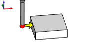
This cycle measures a planar surface face which is parallel to the Y Axis. This cycle can utilize the following geometry inputs: 

 

• Line parallel to the Y Axis.
• Planar surface edge parallel to the Y Axis.
• Planar surface face whose normal is parallel to the X Axis.

Navigation

To access the X Single Surface cycle:

 

1. In the CAM Tree, locate the desired Machine Setup for the Probing cycle, right-click the Machine Setup, and select Probing.
   
   The Probing dialog launches in the Data Entry Manager.
   
   
2. Click the Operations(s) tab.
   
   
3. Click the Parameters tab.
   
   By default the Selected Geometry list is given focus to allow you to select geometry from the graphics area.
   
   
4. Select the applicable geometry.
   
   The geometry is added to the Selected Geometry list and the Initial Position and Parameters section are populated.

 

Note: Some geometry may be applicable to several cycles. In these cases the cycle that is selected based on the geometry may not be the intended cycle. In these cases, simple choose the correct cycle from the drop down list.

The Data Entry Parameters

 

Quick Steps - X Single Surface

 

1. In the CAM Tree, locate the desired Machine Setup for the Probing cycle, right-click the Machine Setup, and select Probing.
   
   The Probing dialog launches in the Data Entry Manager.
   
   
2. Update the Material Approach and Feature Parameters as necessary.
   
   
3. Click the Operations(s) tab.
   
   
4. On the Probe page, select, or define, the Probe to be used.
   
   
5. Click the Parameters tab.
   
   By default the Selected Geometry list is given focus to allow you to select geometry from the graphics area.
   
   
6. Select the desired piece(s) of geometry.
   
   The geometry is added to the Selected Geometry list and the Initial Position and Parameters section are populated.

 

Important: The available cycles are filtered by the geometry selected. If you selected geometry and do not have the desired cycle available, remove the geometry and reselect geometry compatible with the cycle.

7. Update the Initial Position and Parameters sections as needed.
   
   
8. Click the Options tab and update any options necessary.
   
   
9. Click OK.

Example - X Single Surface

In this example we:

 

• Select the Probe feature.
• Select a probe for the cycle.
• Update the Machining Data and Feed groups.
• Select the cycle.
• Adjust the Initial Position.
• Utilize the Options page.
• Backplot the result.

 

Part 1) Selecting the Probe feature

The first step of any Probing cycle is to create a Probing feature in the Machine Setup it is intended to be used in.

 

1. In the CAM Tree, locate the desired Machine Setup for the Probing cycle, right-click the Machine Setup, and select Probing.
   
   The Probing dialog launches in the Data Entry Manager.

 

Note: While the Material Approach and Feature Parameters are available on the initial page of the Probing dialog, those inputs do not apply to this cycle.

Part 2) Selecting the Probe

Selecting a probe can be done with the following steps, or by simply deselecting the System Tool check box and inputting the appropriate data into the required fields.

1. By default Measure is already in the Current Operations list. This will give us access to all available measure cycles in the Operation(s) tab.
   
   At the top of the dialog, click the Operation(s) tab.
   
   
2. By default the Probe page is active. In this page, click the Tool Crib button.
   
   The Tool Crib dialog launches.
   
   
3. Select your probe from the Tool Crib.
   
   
   1. If a probe has not yet been added to your Tool Crib, select the Add From Tool Library button and select one.
      
      
   2. If a probe has not yet been added to your Tool Library, select the Add button, define the probe in the Tool Parameters section, and select OK.
      
      The probe is added to the Tool Library and is automatically highlighted.
      
      
   3. Click OK.
      
      The probe is updated in the dialog.

Part 3) Updating the Machining Data and Feed groups

When selecting a tool from the Tool Crib, a tool number, and the Height and Diameter Offsets should already be correct. However, if you need to update them, you can do that in the Machining Data group. The Feed group will allow you to set a Protected Feedrate for the probe.

1. Update the Machining Data as needed: 
   
   
   1. Update the Tool Number if needed.
      
      
   2. To have the cycle update the Height and Diameter Offset, select the Override Offset button and enter the values to update the offsets to.
      
      
2. Update the Protected Feedrate in the Feed group as needed.

Part 4) Selecting the Cycle

The cycle can be selected with the drop down list under the Cycles section, but simply selecting the appropriate geometry will usually select the required cycle automatically. Since certain geometry could be applicable to several cycles, in some cases, the list will become much smaller. In this case however, there is only one cycle possible for the geometry we choose.

1. Click the Parameters tab.
   
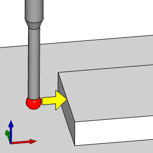
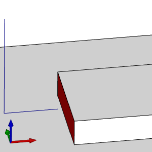
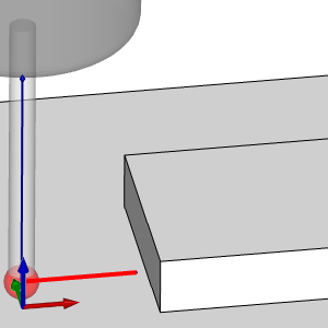
   By default the Selected Geometry list is given focus to allow you to select geometry from the graphics area.
   
   
2. Select a planar surface whose normal is parallel with X, or the edge of that surface.
   
   
   
   The geometry is added to the Selected Geometry list, the Initial Position and Parameters section are populated, and the toolpath becomes visible.
   
   

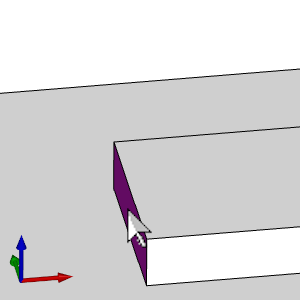
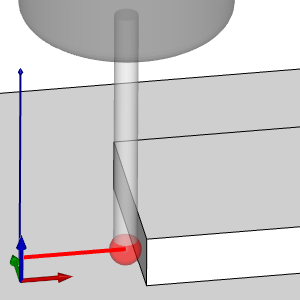
Part 5) Adjusting the Initial Position

There is quite a bit of logic that goes into creating the initial position for you based on the geometry, and the cycle that you choose. While the initial position does not need to be adjusted in this case, we will play with a few of the values to explore how the toolpath reacts.

1. In the Initial Position group, update the X value by adding -0.5 to the end, and pressing Tab.
   
   
   
   The value and the toolpath update to put the initial position of the probe a half inch further back in X.
   
   
2. In the Initial Position group, update the Y value by adding -0.5 to the end, and pressing Tab.
   
   
   
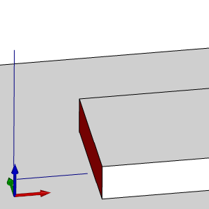
   The value and the toolpath update to put the initial position of the probe a half inch further down in Y.

 

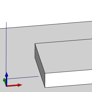
Note: Since our toolpath is shown on the proper side of the surface, we have no need for the Other Side button in this group.

Part 6) Utilizing the Options page

The values in the Options page should only be utilized if you are familiar with exactly how the individual options work.

1. Click the Options tab.
   
   
2. Update any and all options that are needed for the cycle.
   
   
3. Click OK to exit the dialog.
   
   
   
   The dialog closes and the Probing feature is added to the CAM Tree.

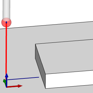
Part 7) Backploting the result

The Backplot is a great way to verify the movements of any of the operations you create.

1. In the CAM Tree, right-click the C Measure operation in the Probing feature and click Backplot.
   
   The Backplot dialog launches.
   
   
2. Click Next to view the probe movements.
   
   
   
   
3. Click Close.
   
   The dialog is closed and the feature is ready to post.